The paper

1. Introduction

A galaxy survey measures a density field through an instrument, an atmosphere and a galaxy. Every one of them leaves a pattern: the survey is deeper in some places than others, dust dims some directions, stars contaminate target selection, seeing varies from night to night, and the telescope scans in stripes. The standard remedy is to regress the observed density against maps of these conditions — templates — and subtract the fit, or equivalently to weight by its inverse [ross2012, ho2012, kitanidis2020]. The regressor has moved from linear models to random forests and neural networks [rezaie2020, chaussidon2022, rezaie2024].

The difficulty is that the correction only ever sees the contaminated data. A regressor that predicts the observed map from the templates will absorb anything the templates can explain — including any part of the true signal that happens to resemble them. This is well known for template projection, whose bias on the power spectrum can be computed [leistedt2014, elsner2016], and it is a named concern for large-scale signals under flexible correction [rezaie2021, rezaie2024]. What is missing is a controlled answer to the question that matters for choosing a method: how does the flexibility of the corrector trade contamination removal against preservation of the signal, and would the standard validation tools notice when it goes wrong?

A cleaner-looking corrected map does not answer this. A map that has lost signal also has less variance, and so looks cleaner. On real data there is no reference to compare against. DarkSignal therefore makes simulation the primary evidence: every world keeps its signal, contamination and noise separately, and every correction is decomposed against them. Real data enters second, as a case study that measures disagreement between methods and, through injection, the one quantity on real systematics whose true value is known.

Our contributions are:

1. Signal–systematic correlation as an exact, swept axis. For any signal family, exactly ρ² of the signal variance lies in the span of the templates. Linear template regression therefore has a closed-form transfer of 1 − ρ², which the benchmark reproduces and uses as an internal check.
2. A decomposition that separates forced from chosen loss. Splitting the signal into its template-orthogonal part s⊥ and template-degenerate part s∥ gives every method two numbers. We show the natural three-way regression fails its own anchor and why.
3. Capacity ladders across method families on one frontier, with oracle ceilings, negative and positive controls with pass thresholds fixed in advance, and spatial cross-validation run both honestly and leakily.
4. An account of why flexible correctors erase signal, separable into two mechanisms, confirmed by a new-sky deployment test, and a mitigation.
5. A real-data case study on the public DESI DR9 target-selection maps, including an injection test on real imaging systematics.

Nothing here measures dark energy, dark matter, or any cosmological parameter.

2. Related work

Survey systematics. Template regression and weighting against stellar density, extinction, seeing and depth are standard in large-scale-structure analyses [ross2012, ho2012]. For DESI, target densities have been correlated with Legacy Surveys imaging conditions [kitanidis2020, dey2019], and the target-selection pipeline that produces the maps used here is described by [myers2023]. Extinction templates derive from the SFD dust map [sfd1998].

Bias from projection. Marginalising over known modes goes back to giving them infinite variance [rybicki1992], and was used for foreground marginalisation in CMB likelihoods [slosar2004]. Mode projection and template subtraction bias clustering estimates low when chance correlations exist between the signal and the templates; the bias can be computed and removed [leistedt2014, elsner2016]. [weaverdyck2021] compare mitigation methods on simulations with known contamination. Our closed form 1 − ρ² is the controlled, variance-level version of the projection bias, with ρ set exactly instead of arising by chance.

Machine-learned correction. Neural-network weights on Legacy Surveys imaging [rezaie2020], random-forest weights for DESI quasar targets on DR9 [chaussidon2022], and flexible mitigation for large-scale signals such as primordial non-Gaussianity, where over-correction of large scales is an explicit concern [rezaie2021, rezaie2024]. These analyses validate on mocks; we sweep the flexibility itself.

Component separation. CMB foreground cleaning faces the same trade-off with multiple frequencies: internal linear combinations carry a known bias from chance signal–foreground correlation [tegmark2003], and independent pipelines are compared on the same data [planck2020comp], which is the practice our real-data section follows. ICA has been applied to astrophysical component separation [maino2002, hyvarinen2000]. The transfer-function estimator we use for scale-resolved retention is the simulation-calibrated one familiar from CMB power-spectrum work [hivon2002].

Outside astronomy. Nuisance regression that removes and distorts the signal of interest is documented in fMRI [murphy2009, lindquist2019], and adjusting for a variable on the path of the effect biases it toward zero in epidemiology [schisterman2009]. We use these as analogies only. Random splits of spatially autocorrelated data give optimistic validation scores [roberts2017, ploton2020]. Self-supervised denoisers assume noise independent across pixels [batson2019, lehtinen2018, vincent2008], an assumption spatially coherent contamination violates. The capacity ladders are an L-curve [hansen1992] in a different pair of axes.

3. Problem definition

An observed map is

d = s + c + n,

with s the signal, c the contamination and n unit-variance noise, so the signal amplitude is the signal-to-noise ratio. A corrector receives d, a template matrix T whose columns are the maps of observing conditions the analyst holds, and a mask, and returns ŝ. It never sees s, c or n; the two oracle correctors that do are labelled and excluded from every claim about deployable methods.

Let B be an orthonormal basis of the column space of the true templates, and split

s = s_⊥ + s_∥, s_∥ = B B^ᵀ s.

s∥ is the part of the signal any template-based correction can mistake for contamination; s⊥ is the part none can. The signal–systematic correlation is defined by ρ² = Var(s∥) / Var(s).

4. Simulation

Worlds are periodic 64 × 64 grids (32² and 128² in the sample-size slice). Six synthetic templates stand in for depth, extinction, stellar density, seeing, airmass and scan stripes. They are smooth, and two are deliberately degenerate. Four signal families cover a power-law Gaussian field, a log-normal clustered field, a field with a narrow spectral feature, and sparse localised events on a weak background. Six contamination families cover linear, nonlinear (saturating, quadratic and interaction terms), stripe-dominated, depth-multiplicative, localised artefacts, and a half-unmodelled case in which half the contamination has no template at all.

The ρ construction. A drawn signal is rebuilt as

s = σₛ(√(1−ρ²) u + ρ v),

where u is the drawn field with its template-span component removed and v is a random unit direction inside the span, both standardised. Exactly ρ² of the variance lies in the span; the test suite verifies it to 10⁻⁹ for every family. Any correction that projects out the span loses s∥ entirely, so linear regression's signal transfer is exactly 1 − ρ².

Grid. The canonical world is a power-law signal, linear contamination at amplitude 1.5, medium SNR (signal s.d. 1.0), ρ = 0.3. Slices vary one or two dimensions around it: ρ ∈ {0, 0.1, 0.2, 0.3, 0.5, 0.7}; SNR ∈ {2, 1, 0.5, 0.2}; all signal × contamination families; capacity ladders; four controls; cross-validation; distribution shift on the same sky and on a new sky; template ablation and spurious templates; sample size; masks and depth-dependent noise. The STANDARD grid has 9,742 runs over 55 world configurations, with 0 failures. Every run records its configuration, method, hyperparameters, metrics, runtime and git commit.

5. Correction methods

No correction; ordinary least squares (and a degree-2 variant); ridge; lasso; PCA and ICA on the templates followed by least squares; RBF kernel ridge (a Gaussian-process posterior mean, fitted on a pixel subsample); random forest; histogram gradient boosting; an MLP; a CNN that regresses the observed map on the template maps with circular padding; a patch autoencoder trained on the observed map itself, with no templates, whose reconstruction is subtracted; subspace projection as an analytic reference; and two oracles, the best linear fit to the true contamination and the true contamination itself. The CNN never receives the observed map as input: given it as both input and target, a CNN learns the identity. No transformer is included; the data have no sequence structure and a few thousand pixels per world.

Every method except the fixed ones has a capacity ladder from rigid to clearly over-flexible — ridge and lasso penalties, components, kernel penalty, tree depth, boosting iterations and leaves, hidden widths, CNN channels and depth, autoencoder bottleneck. Numerical libraries are pinned to one thread: on the development machine one gradient-boosting fit took 0.41 s single-threaded and 44 s at the default thread count.

6. Metrics

Why the obvious decomposition fails. Regressing ŝ on (s, c, n) seems natural. When s∥ and c share a subspace, least squares can explain away genuine loss by borrowing from the contamination coefficient: on a world where linear correction provably destroys 36% of the signal variance (ρ = 0.6), it reports a transfer of 0.81.

The split decomposition. We regress ŝ on [s⊥, s∥, c, n]. Because s⊥ is orthogonal to s∥ and to any contamination inside the template span, its coefficient is well identified. The coefficients are the clean transfer (on s⊥: below 1 is erasure the method chose), the degenerate transfer (on s∥), the contamination leakage (on c; contamination removed = 1 − leakage) and the noise transfer. The residual variance relative to the signal variance is unexplained structure. That term includes invented structure, but also contamination that was removed along some directions and survives with a changed shape. The total signal transfer recombines the two signal terms, (1 − ρ²)·clean + ρ²·degenerate. Three anchors are asserted in the tests: no correction gives transfer 1 and leakage 1; the oracle gives 1 and 0; linear regression gives 1 − ρ².

Scale-resolved retention uses the cross-spectrum transfer T(k) = Re⟨ŝ s*⟩ / ⟨|s|²⟩, in 12 log bins, summarised as large-scale (k < 6) and small-scale (k ≥ 6) means. Anomaly retention is aperture flux at the known event positions relative to truth. An aggregate loss, leakage² + (1 − transfer)² + unexplained, is reported for ranking only; the three components are always shown and the weights are swept.

Statistics. The unit of replication is the world. Differences between methods are computed within world and summarised by 95% percentile bootstrap intervals over seeds (10,000 resamples), with Wilcoxon signed-rank tests and Holm correction. Where a slice had five seeds, a 5-pair Wilcoxon test cannot fall below p = 0.0625, so no rule demanding p < 0.05 was decidable there. Those slices were extended to 10 and 15 seeds with the rules unchanged (decision log D19).

7. Controls

Four controls, with thresholds fixed before results. Zero contamination: there is nothing to remove, so a safe method keeps signal transfer ≥ 0.95. Spurious templates: no contamination, three smooth templates with no causal role; same threshold. Strong contamination: amplitude 4, ρ = 0; a useful method removes ≥ 0.80. Adversarial: ρ = 0.7, not graded; it shows the forced loss.

8. Results

8.1 The closed form holds

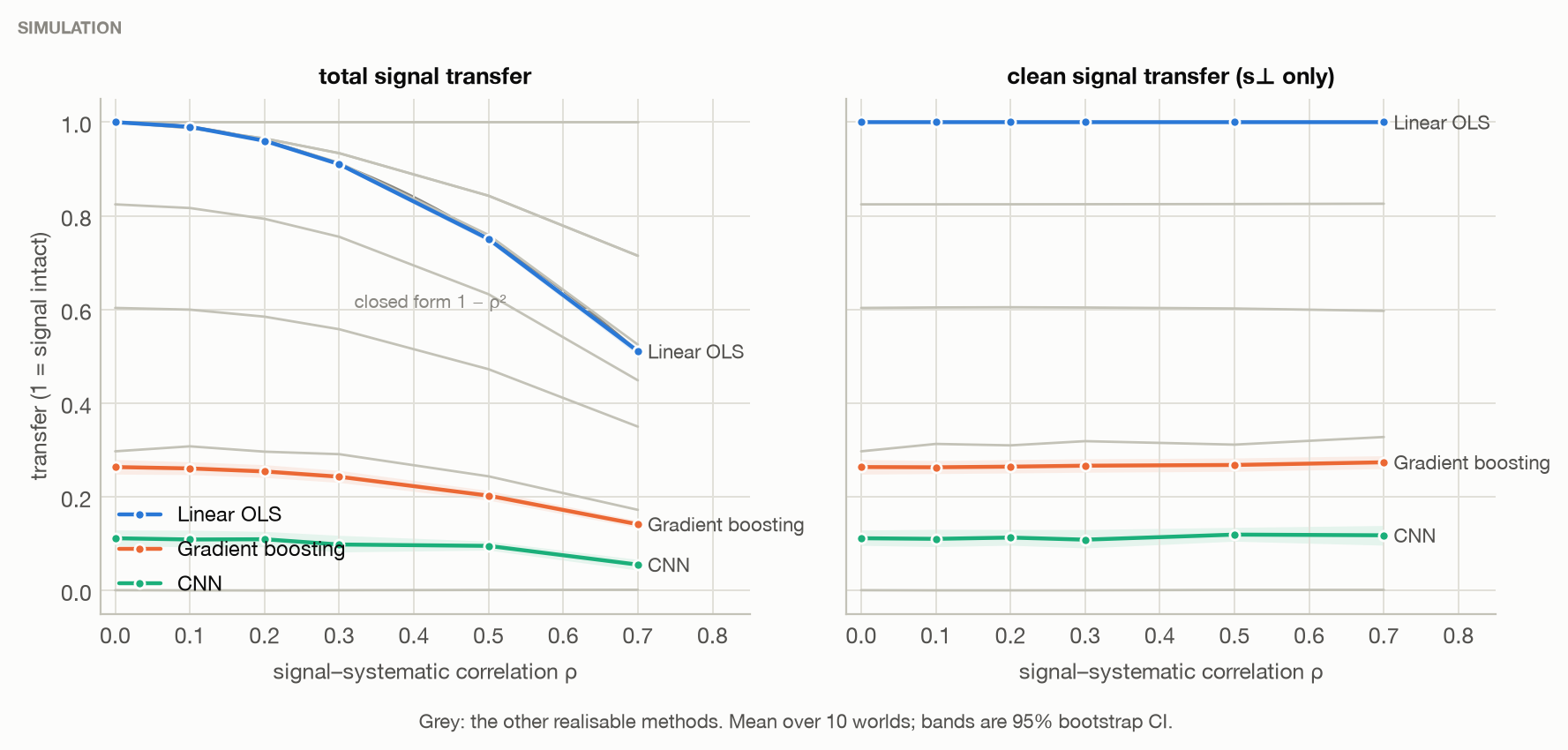
Linear regression's total transfer matches 1 − ρ² to within 0.0006 across the ρ sweep. Its clean transfer is 1.000: everything it loses, the degeneracy forced. PCA and ICA agree to 4e-15 in every world. That is not a coincidence: FastICA whitens into the leading PCA subspace and rotates within it, and least-squares subtraction does not change under rotation, so ICA's independence assumption buys nothing for linear template subtraction.

8.2 Flexibility buys removal and costs signal

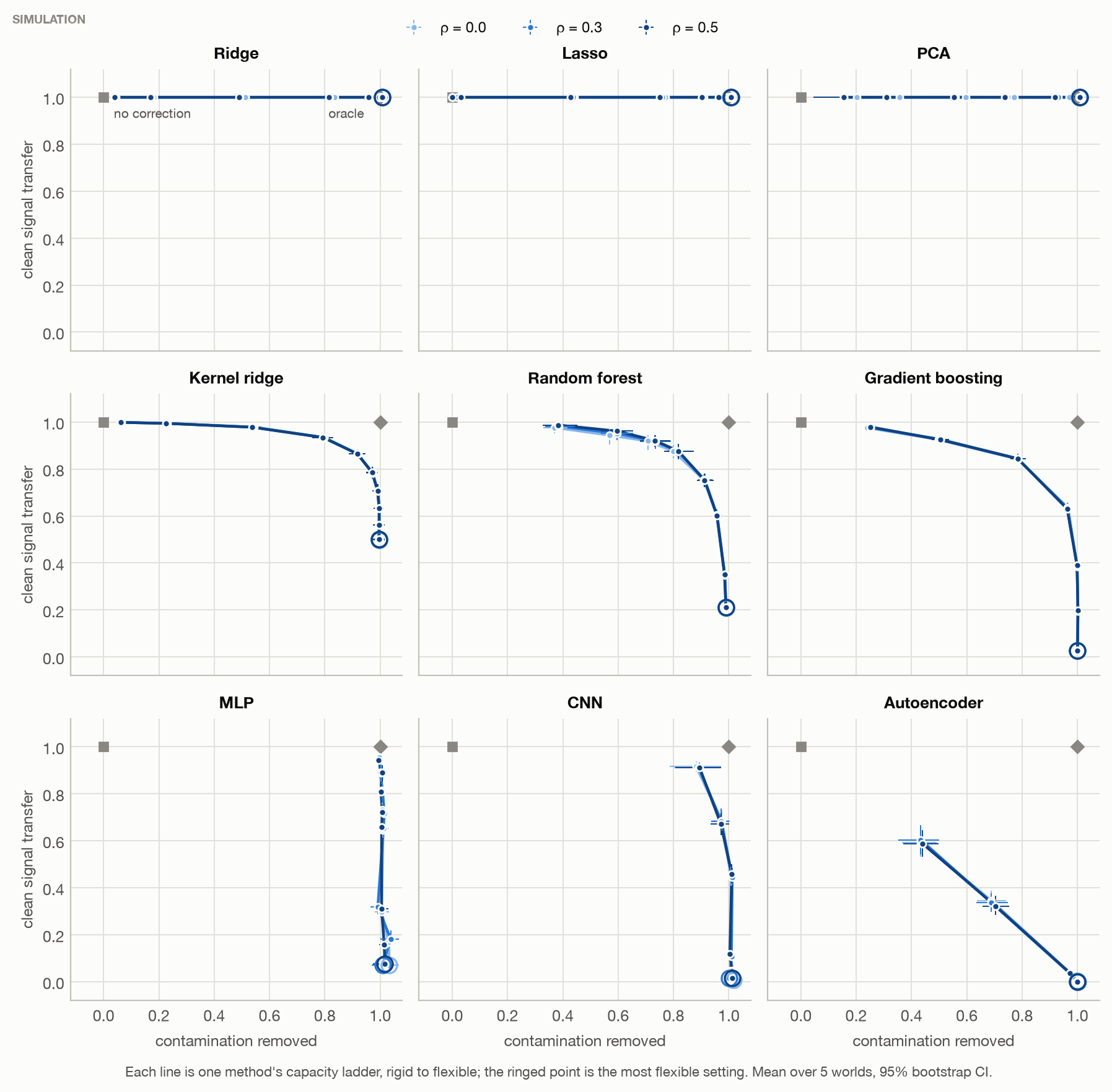
On nonlinear contamination families, flexible correctors remove more contamination than linear regression (H1, supported). For gradient boosting the paired difference is +0.39 (Holm p = 7e-12, n = 40); random forest, MLP and CNN are similar. The price is signal. At the canonical world gradient boosting keeps 0.27 of the clean signal, the MLP 0.32, the random forest 0.60, kernel ridge 0.82, the CNN 0.11 and the autoencoder 0.00. Along each ladder, clean transfer falls as capacity rises. The linear family runs along the top of the frontier because it can only remove what the templates span.

Across every contaminated world in the ρ, SNR, family, sample-size and observing-condition slices, the linear family is "safe" (clean transfer ≥ 0.90 and removal ≥ 0.80) in 8e+01% of worlds; every flexible method is safe in none. Rankings by aggregate loss are only moderately stable across worlds (Kendall's W = 0.63), and the best method changes with the loss weights. The components, not the aggregate, carry the conclusion.

8.3 The erasure is not caused by correlation

H2 predicted that flexible methods erase more signal than rigid ones at matched removal, increasingly so as ρ grows. At matched removal of 0.90 they do erase more. But the gap does not grow: for gradient boosting the change from ρ = 0 to ρ = 0.5 is +0.002 [-0.019, +0.026], and the same holds at matched removal of 0.80 and 0.95 (H2, refuted). Clean transfer is flat in ρ for every method. Whatever a flexible corrector erases beyond the forced loss, it erases whether or not the signal resembles the templates.

8.4 Negative controls expose every flexible method

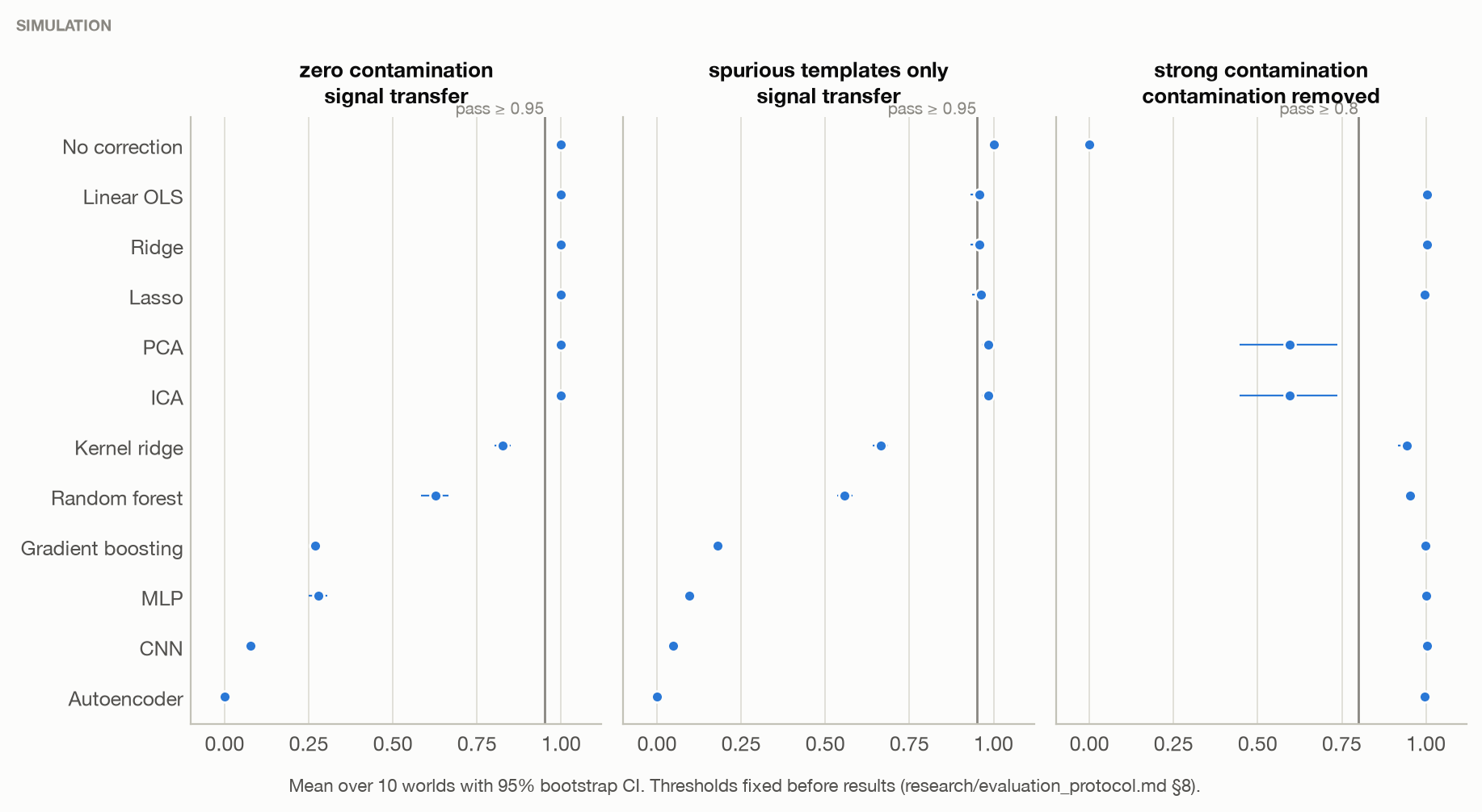
With zero contamination, linear regression keeps 1.000 of the signal and passes in 1e+02% of worlds. Gradient boosting keeps 0.27, the MLP 0.28, the random forest 0.63, kernel ridge 0.83, and all pass in 0% of worlds. With three irrelevant templates, linear regression still keeps 0.958. All realisable methods except PCA and ICA (which use only three components) pass the strong-contamination control.

8.5 Weak signals and small maps

Ridge has a lower aggregate loss than every flexible method at low and extreme-weak SNR and on 32 × 32 maps (H5, supported). On the smallest maps gradient boosting's excess loss over ridge is 0.87 (n = 15, Holm p = 7e-04). Clean transfer for gradient boosting rises from 0.10 at 32² to 0.38 at 128². More pixels per fit means less memorisation, but even at 128² the gap to linear is large. Localised events fare worst: gradient boosting keeps 0.26 of their aperture flux and the CNN 0.03, against 1.02 for linear regression.

8.6 Erasure concentrates at large scales

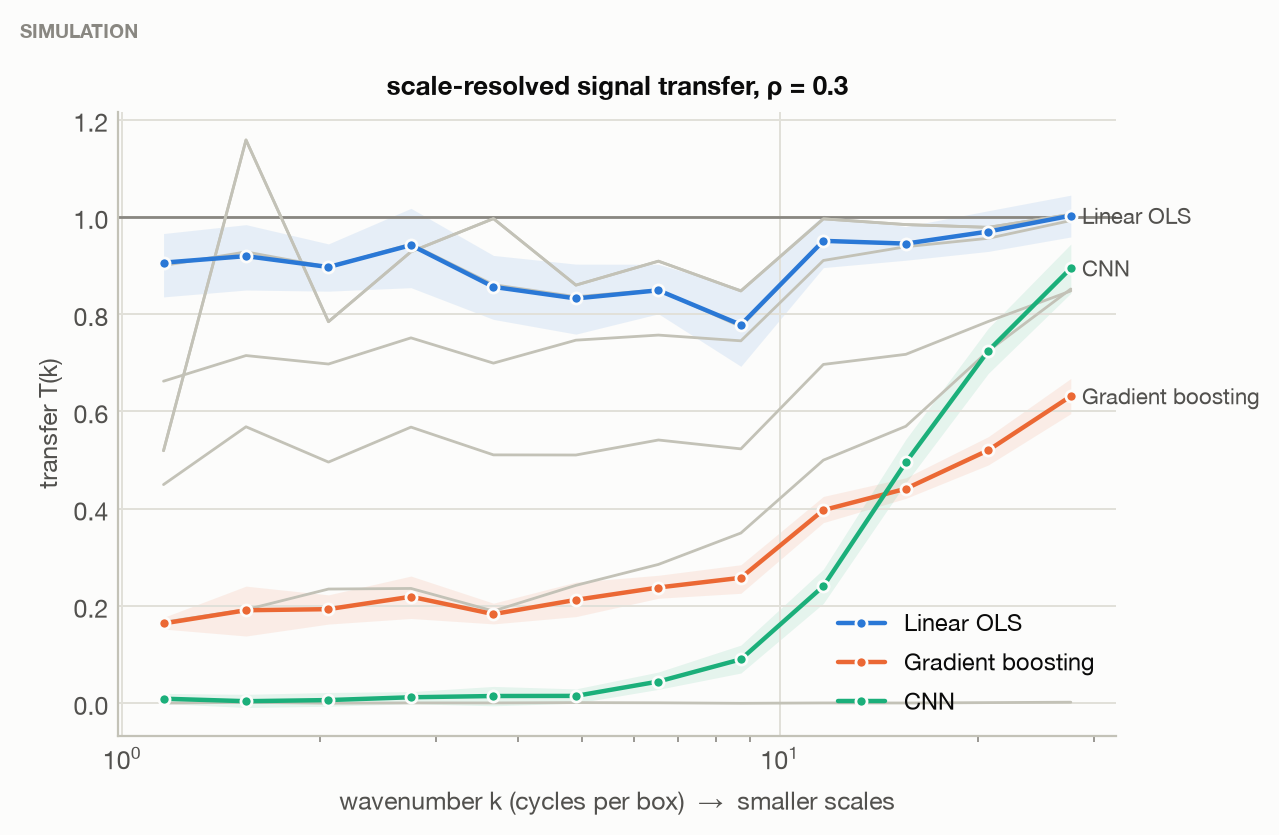
Large-scale transfer is below small-scale transfer for linear regression (difference -0.045) and far more so for flexible correctors — -0.39 for the CNN, -0.32 for the MLP, -0.22 for gradient boosting (H6, supported). In the clustered family the two-point correlation of the corrected map is 0.06 of the truth for gradient boosting, against 0.84 for linear regression.

8.7 Would cross-validation have warned you?

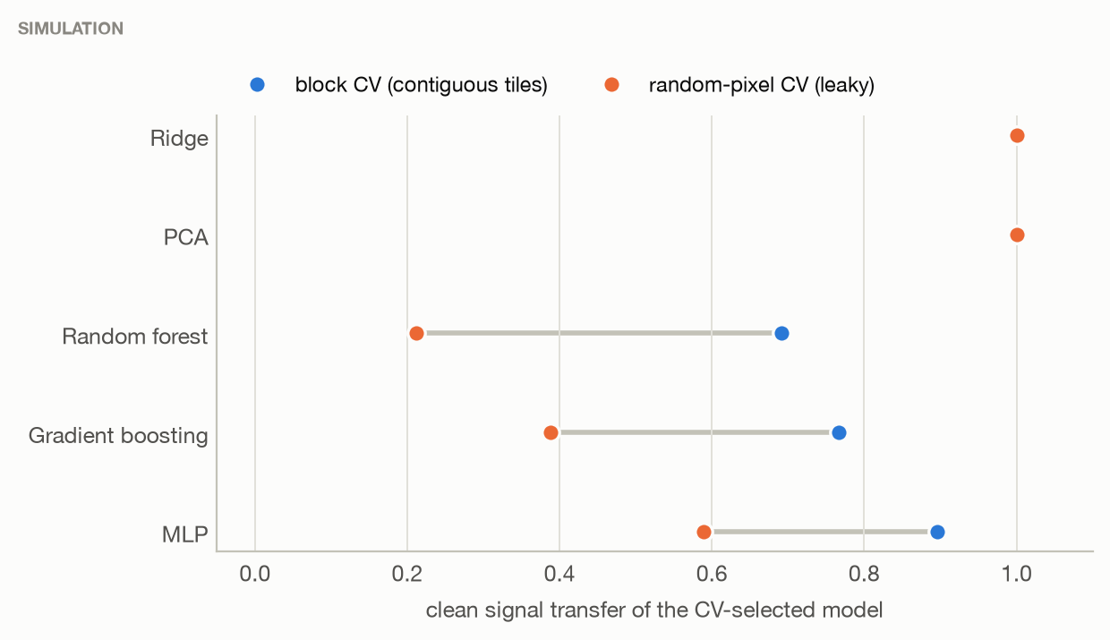
Block cross-validation ranks the methods correctly. Every method that fails the zero-contamination control has a lower canonical block-CV R² than the best method that passes it (0.435), so H4 — that controls catch what validation misses — is refuted as registered. Along each ladder, the block-CV choice lies within one rung of the rung that minimises aggregate loss in all but 1e+01% of flexible-method worlds (H3, refuted under the decisive operationalisation, decision log D14).

Two qualifications carry the practical message. First, the size of the warning is small next to the size of the damage. The autoencoder removes all of the signal and scores a block-CV R² of 0.396, against 0.432 for ridge. Second, the fold scheme decides everything. Random-pixel folds rank gradient boosting (R² 0.592) above ridge (0.528), and select models that keep 0.21 of the clean signal for the random forest, where block folds select one that keeps 0.69.

8.8 Uncertainty flags the risky corrections

For five correctors at three capacities, we trained five-member ensembles, each on a random 75% of the spatial blocks with its own seed. Ensemble spread needs no ground truth, yet across 168 (method, capacity, world) points its rank correlation with excess signal loss is 0.89. Pixel by pixel, disagreement between methods correlates with the true error at 0.42 on average. Spread and erasure plausibly share a cause — a model that fits its training pixels closely is also sensitive to which pixels it was given — so this is a useful warning, not a calibrated error bar.

9. Overcorrection: two mechanisms and a mitigation

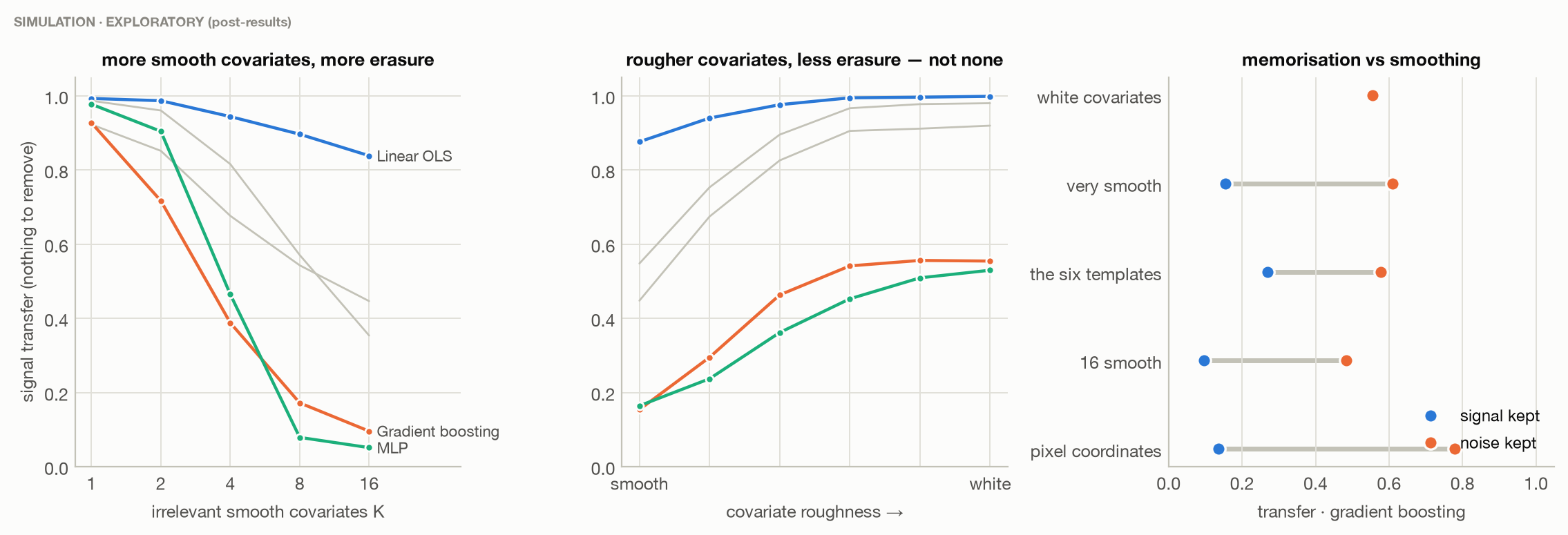
Why would a corrector remove signal uncorrelated with every template, from data with nothing to remove? This section is exploratory and was designed after the canonical results were read (decision log D18). On zero-contamination worlds we changed only the covariates the corrector receives.

Memorisation. Handed six spatially white covariates, gradient boosting keeps 0.55 of the signal and 0.55 of the noise — identical, and flat across scales. A flexible model fitted and applied on the same pixels partly reproduces them, signal and noise alike.

Covariates as coordinates. Handed explicit pixel coordinates, it keeps 0.14 of the signal but 0.78 of the noise, and 0.02 of large-scale signal against 0.52 of small-scale. Smooth covariates vary slowly across the map, so a flexible function of them is a spatial smoother of the observation. Erasure grows with the number of irrelevant smooth covariates (0.93 kept with one, 0.10 with sixteen) and with their smoothness. Real nuisance templates are smooth, so they do both.

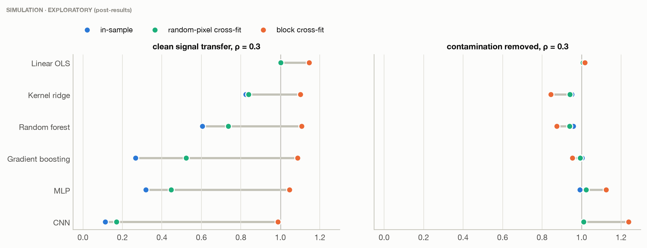
Confirmation from a new sky. If the erasure comes from correcting the map a model was fitted on, a correction trained on one sky and applied to another should not erase the second sky's signal. With the instrument's systematic response held fixed and a different sky for training, gradient boosting's clean transfer on the test sky is 1.06, the MLP's 1.06 and the CNN's 0.98. They also remove more same-family contamination than linear regression (0.86 and 0.93 against 0.73). Trained and applied on the same sky, gradient boosting keeps 0.27.

Mitigation. A survey cannot train on another sky with the same systematics, but it can refuse to correct any pixel with a model that saw it. Under block cross-fitting — fit on three of four folds of contiguous tiles, apply to the fourth, rotate — gradient boosting's clean transfer at the canonical world goes from 0.27 to 1.09, while contamination removed goes from 1.00 to 0.95. For the MLP the same numbers are 0.32 → 1.05 and 0.99 → 1.12. On the zero-contamination control, cross-fitted gradient boosting keeps 1.08 of the signal. Cross-fitting over random pixels instead of blocks helps only partly (gradient boosting 0.52): it stops memorisation, but neighbouring pixels still let the model smooth the map. That separates the two mechanisms a second way.

Block cross-fitting is a trade, not a cure. Clean transfer now overshoots 1 for every method, linear regression included (1.15). A fit that leaves a block out is biased against that block's own signal, so subtracting it adds a little of the signal back. Our ρ construction makes s⊥ exactly orthogonal to the templates over the whole map, which exaggerates this overshoot relative to a real survey. Removal also falls for the tree methods (random forest 0.96 → 0.87) and overshoots for the CNN (1.24). On the real DESI templates, block cross-fitting raises gradient boosting's clean transfer of the injected field from 0.859 to 0.974. Cross-fitted, it removes almost none of the real map's variance (0.998 survives, against 0.788 in-sample and 0.956 for linear regression). That is consistent with its near-zero block-CV R²: most of what it removed in-sample did not generalise across the sky.

10. Generalisation

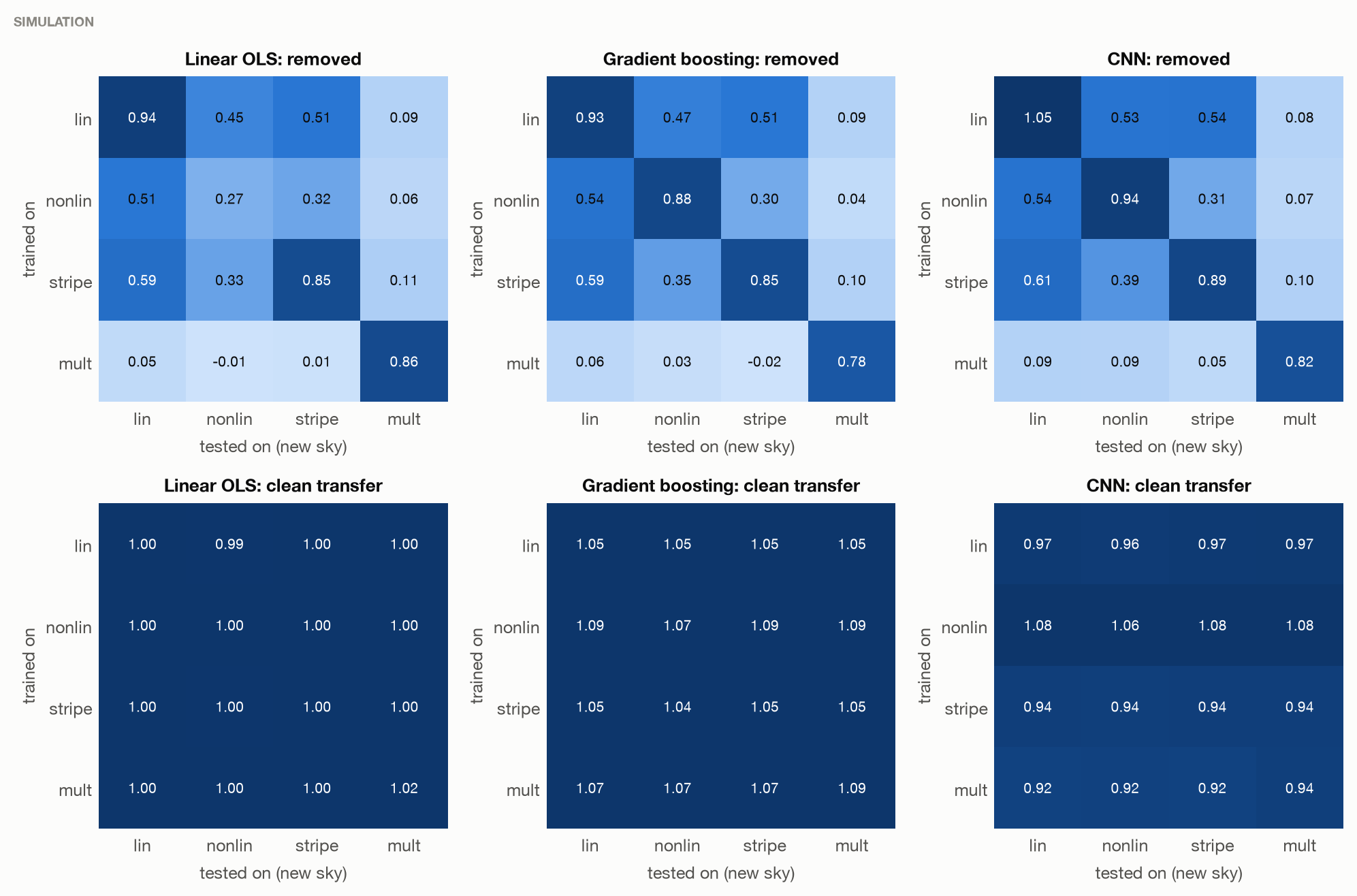
Deployed under a different contamination regime on the same sky, every method's removal collapses (linear regression removes 0.10, gradient boosting 0.10). On a new sky with a different contamination family, removal is also low for every method (linear 0.25, gradient boosting 0.25). A correction learned for one systematic response does not transfer to another, flexible or not. Dropping a causal template costs linear regression more removal than it costs gradient boosting, since the tree can partly reconstruct the missing driver from correlated templates. Adding irrelevant smooth templates costs flexible methods signal, which is what the coordinates mechanism predicts. When the analyst's templates carry measurement noise equal to their own standard deviation, linear regression still never erases signal (clean transfer 1.00) but removes only 0.45 of the contamination — the errors-in-variables attenuation. Gradient boosting removes 0.71 and keeps 0.53 of the clean signal: noisy covariates are rougher, so it smooths less, as the coordinates mechanism predicts.

11. Real-data case study

Data. We use the public DESI DR9 target-selection pixweight map for the main dark-time survey (Early Target Selection release; desitarget 0.49.0; sha256 verified against the published checksum; CC BY 4.0). It gives, per nside-256 HEALPix pixel, the density of DESI luminous red galaxy (LRG) targets and the imaging conditions there [myers2023, dey2019]. We degrade to nside 128 with FRACAREA weights and keep pixels with FRACAREA ≥ 0.9, E(B − V) < 0.15 and Dec < 32.375°. That leaves 67,180 pixels, about 14,100 deg². The target is the LRG density contrast. The twelve templates are stellar density, E(B − V), PSF depth in g, r, z and W1, galaxy depth in g, r and z, and PSF size in g, r and z. The CNN and autoencoder are omitted because they assume a planar grid. No corrected map here is ground truth.

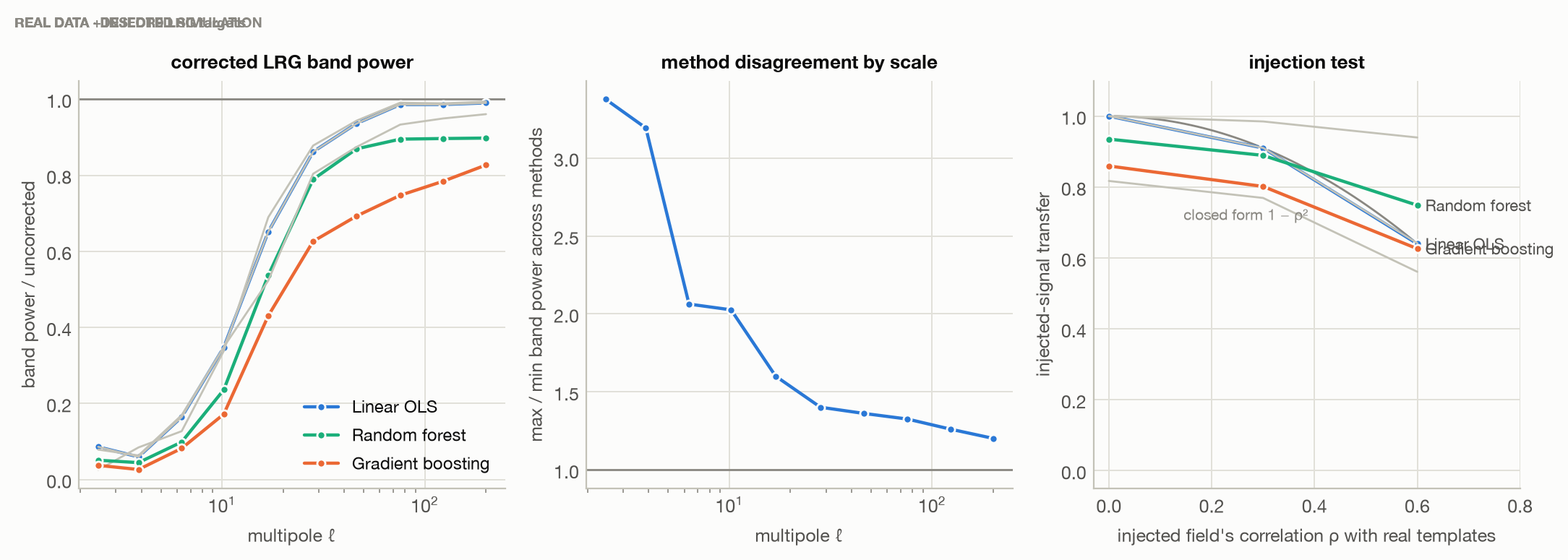
What the correctors do. Linear correction removes every template correlation by construction and 0.956 of the variance survives it; after gradient boosting, 0.788 survives. Block cross-validation on nside-4 superpixels gives R² = 0.043 for linear regression, 0.020 for the random forest, 0.002 for gradient boosting and -0.055 for the MLP. The flexible models remove more variance and generalise worse between regions of sky. Every corrector removes most of the lowest-multipole power: at 2 ≤ ℓ < 3, linear correction keeps 0.086 of the uncorrected band power. Large-scale LRG target density is dominated by systematics there, so this is expected; how much of it was signal cannot be known from these data. At 22 ≤ ℓ < 36, linear correction keeps 0.86 and gradient boosting 0.63.

Where they disagree. Across the six corrections, the largest and smallest band power differ by a factor of 3.4 at 2 ≤ ℓ < 3 and 1.20 at 157 ≤ ℓ < 256. Large scales, where the science of primordial non-Gaussianity lives, are exactly where the answer depends on the corrector.

Injection. We add a simulated field with exact correlation ρ to the real templates, correct with and without it, and project the difference on the injected field. Linear correction transfers 0.910 of it at ρ = 0.3 and 0.640 at ρ = 0.6 — the closed form gives 0.910 and 0.640 — so the degeneracy bound holds on real imaging systematics. Gradient boosting transfers 0.859 of the injected signal's clean part at every ρ: on real data too, flexible correction erases a ρ-independent share of a signal it had no reason to touch. That share is smaller than in simulation, consistent with 67,180 pixels per fit rather than 4,096.

12. Limitations

The simulations are flat, periodic, two-dimensional and noise-Gaussian, with synthetic templates supplied without measurement error; real templates are estimates and would add errors-in-variables bias. The degenerate component of the signal is a random direction in the template span, whereas a real chance correlation has specific structure; the closed form does not depend on the direction, but flexible methods might. Capacity ladders are finite and hand-chosen, and each neural family is one architecture. The distortion term counts reshaped residual contamination as unexplained. The mechanism, new-sky and mitigation analyses were designed after the canonical results and are exploratory. On real data there is no truth. The pixweight map gives target densities rather than a redshift-resolved sample, the band powers are pseudo-C_ℓ without mask deconvolution, only the southern imaging region is used, and the MLP was capped at 150 iterations for runtime. The full list, with each item's status, is in research/limitations.md.

13. Conclusion

A cleaner map is not a truer map. When the signal shares structure with the templates, any template-based correction loses exactly the shared part, and the loss has a closed form that holds in simulation and on real DESI imaging systematics. Flexible correctors remove more contamination and also erase signal that no template could mimic. The cause is not that correlation but correcting the map they were fitted on, which a zero-contamination control exposes in one run. Block cross-validation ranks methods correctly but understates the damage, and random-pixel validation selects the most harmful models. We recommend that every machine-learned systematics correction report a zero-contamination control and an injection test, validate with spatial blocks, and prefer corrections that are not applied to the pixels they were fitted on — while checking, with the same controls, that out-of-sample fitting has not introduced a bias of its own.

Data and code availability

All code, protocols, the registered hypotheses, the decision log and every canonical result file are in the DarkSignal repository; make reproduce regenerates them. Canonical results: git dbc5242cfe0917923a2255b71e4f6ca181afe4d8. The DESI data are public (CC BY 4.0).

Acknowledgments

This research used data obtained with the Dark Energy Spectroscopic Instrument (DESI). DESI construction and operations is managed by the Lawrence Berkeley National Laboratory. This material is based upon work supported by the U.S. Department of Energy, Office of Science, Office of High-Energy Physics, under Contract No. DE-AC02-05CH11231, and by the National Energy Research Scientific Computing Center, a DOE Office of Science User Facility under the same contract. Additional support for DESI was provided by the U.S. National Science Foundation (NSF), Division of Astronomical Sciences under Contract No. AST-0950945 to the NSF's National Optical-Infrared Astronomy Research Laboratory; the Science and Technology Facilities Council of the United Kingdom; the Gordon and Betty Moore Foundation; the Heising-Simons Foundation; the French Alternative Energies and Atomic Energy Commission (CEA); the National Council of Humanities, Science and Technology of Mexico (CONAHCYT); the Ministry of Science and Innovation of Spain (MICINN), and by the DESI Member Institutions: www.desi.lbl.gov/collaborating-institutions. The DESI collaboration is honored to be permitted to conduct scientific research on I'oligam Du'ag (Kitt Peak), a mountain with particular significance to the Tohono O'odham Nation. Any opinions, findings, and conclusions or recommendations expressed in this material are those of the author(s) and do not necessarily reflect the views of the U.S. National Science Foundation, the U.S. Department of Energy, or any of the listed funding agencies.